Who Rewrote My SQL?

There are several new features in Oracle 12c that are implemented under the hood by changing the SQL statement that we write to a different statement (e.g., by adding some hidden predicates).
In OUG Ireland 2016 I talked about two such features – In Database Archiving and Temporal Validity – as part of my “Write Less (Code) with More (Oracle12c New Features)” presentation. I usually talk about another such feature in this presentation – the Row Limiting clause. This time I skipped it, but Tim Hall talked about it two hours later in his “Analytic Functions: An Oracle Developer’s Best Friend” presentation. Following these presentations I had two short and interesting chats with Tim and with Jonathan Lewis about when, during the statement execution, Oracle rewrites the statements in these features. These chats are the motivation for this post.

When a SQL statement is processed, it goes through several stages, in this order: parsing, optimization, row source generation, and execution.

Note: Parsing is a confusing term, as many times when we say “parsing” (especially “hard parsing”) we actually mean “parsing + optimization + row source generation”.

The first stage, the parsing, is not too complex. The Parser basically checks the syntax and the semantics of the statement. If needed, it also expands the statement. For example, it replaces each view referenced in the statement with its definition, so after parsing the statement refers only to actual tables. Another example: it expands * to the actual column list.
The second stage, the optimization, is much more complex. The Optimizer has several components, and the first one is the Query Transformer. This component may further rewrites the SQL statement that it gets from the Parser, but the purpose here is to find an equivalent statement with a lower cost.

In Oracle 12c we have a simple (and documented) way to see the output of the expansion that is done by the Parser – using the DBMS_UTILITY.EXPAND_SQL_TEXT procedure.

Note: to be more precise, I assume that this procedure reveals everything that the Parser does during the expansion stage, and only that. The documentation of DBMS_UTILITY.EXPAND_SQL_TEXT is very limited. It only says “This procedure recursively replaces any view references in the input SQL query with the corresponding view subquery”, and the Usage Notes imply that it also shows the outcome of applying VPD policies.

Row Limiting

Apparently the new Row Limiting clause, used for Top-N and paging queries, is implemented at the expansion stage. We can see that a query that uses the new Row Limiting syntax is expanded to a pre-12c syntax using analytic functions:

var x clob
begin
  dbms_utility.expand_sql_text(
    input_sql_text => '
      select project_id,
             person_id,
             assignment_id,
             assignment_period_start,
             assignment_period_end
      from project_assignments
      order by project_id,person_id
      OFFSET 100 ROWS 
      FETCH NEXT 4 ROWS ONLY',
    output_sql_text => :x);
end;
/
 
print x

-- I formatted the output to make it more readable
SELECT "A1"."PROJECT_ID"              "PROJECT_ID",
       "A1"."PERSON_ID"               "PERSON_ID",
       "A1"."ASSIGNMENT_ID"           "ASSIGNMENT_ID",
       "A1"."ASSIGNMENT_PERIOD_START" "ASSIGNMENT_PERIOD_START",
       "A1"."ASSIGNMENT_PERIOD_END"   "ASSIGNMENT_PERIOD_END"
FROM   (SELECT "A2"."PROJECT_ID" "PROJECT_ID",
               "A2"."PERSON_ID" "PERSON_ID",
               "A2"."ASSIGNMENT_ID" "ASSIGNMENT_ID",
               "A2"."ASSIGNMENT_PERIOD_START" "ASSIGNMENT_PERIOD_START",
               "A2"."ASSIGNMENT_PERIOD_END" "ASSIGNMENT_PERIOD_END",
               "A2"."PROJECT_ID" "rowlimit_$_0",
               "A2"."PERSON_ID" "rowlimit_$_1",
               row_number() over(ORDER BY "A2"."PROJECT_ID", "A2"."PERSON_ID") "rowlimit_$$_rownumber"
        FROM   "DEMO5"."PROJECT_ASSIGNMENTS""A2") "A1"
WHERE  "A1"."rowlimit_$$_rownumber" <= CASE WHEN (100 >= 0) THEN floor(to_number(100)) ELSE 0 END + 4
AND    "A1"."rowlimit_$$_rownumber" > 100
ORDER  BY "A1"."rowlimit_$_0",
          "A1"."rowlimit_$_1"

For more examples like this, and more details about Row Limiting in general, see Write Less with More – Part 5.

Temporal Validity

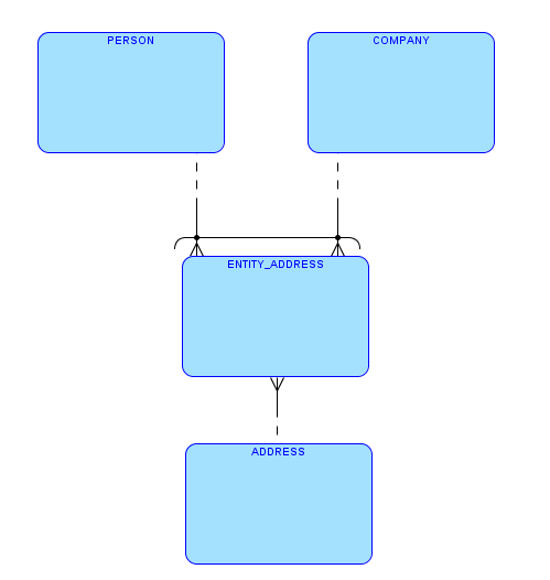
Temporal Validity allows to apply filtering based on validity period (or range), either explicitly or implicitly.
Explicit filtering is done at the statement-level. Implicit filtering is done by a session-level control.
We can see that both statement-level control and session-level control are implemented at the expansion stage:

alter table project_assignments 
       add PERIOD FOR assignment_period;

var x clob
begin
  dbms_utility.expand_sql_text(
    input_sql_text => '
      select person_id,
             project_id,
             assignment_period_start,
             assignment_period_end
      from   project_assignments
      AS OF PERIOD FOR assignment_period SYSDATE',
    output_sql_text => :x);
end;
/
 
print x

SELECT "A1"."PERSON_ID"               "PERSON_ID",
       "A1"."PROJECT_ID"              "PROJECT_ID",
       "A1"."ASSIGNMENT_PERIOD_START" "ASSIGNMENT_PERIOD_START",
       "A1"."ASSIGNMENT_PERIOD_END"   "ASSIGNMENT_PERIOD_END"
FROM   (SELECT "A2"."ASSIGNMENT_PERIOD_START" "ASSIGNMENT_PERIOD_START",
               "A2"."ASSIGNMENT_PERIOD_END"   "ASSIGNMENT_PERIOD_END",
               "A2"."ASSIGNMENT_ID"           "ASSIGNMENT_ID",
               "A2"."PERSON_ID"               "PERSON_ID",
               "A2"."PROJECT_ID"              "PROJECT_ID"
        FROM   "DEMO5"."PROJECT_ASSIGNMENTS" "A2"
        WHERE  ("A2"."ASSIGNMENT_PERIOD_START" IS NULL OR "A2"."ASSIGNMENT_PERIOD_START" <= SYSDATE)
        AND    ("A2"."ASSIGNMENT_PERIOD_END" IS NULL OR "A2"."ASSIGNMENT_PERIOD_END" > SYSDATE)) "A1"
> exec dbms_flashback_archive.enable_at_valid_time('CURRENT')

PL/SQL procedure successfully completed.

var x clob
begin
  dbms_utility.expand_sql_text(
    input_sql_text => '
      select person_id,
             project_id,
             assignment_period_start,
             assignment_period_end
      from   project_assignments',
    output_sql_text => :x);
end;
/
 
print x

SELECT "A1"."PERSON_ID"               "PERSON_ID",
       "A1"."PROJECT_ID"              "PROJECT_ID",
       "A1"."ASSIGNMENT_PERIOD_START" "ASSIGNMENT_PERIOD_START",
       "A1"."ASSIGNMENT_PERIOD_END"   "ASSIGNMENT_PERIOD_END"
FROM   (SELECT "A2"."ASSIGNMENT_PERIOD_START" "ASSIGNMENT_PERIOD_START",
               "A2"."ASSIGNMENT_PERIOD_END"   "ASSIGNMENT_PERIOD_END",
               "A2"."ASSIGNMENT_ID"           "ASSIGNMENT_ID",
               "A2"."PERSON_ID"               "PERSON_ID",
               "A2"."PROJECT_ID"              "PROJECT_ID"
        FROM   "DEMO5"."PROJECT_ASSIGNMENTS" "A2"
        WHERE  ("A2"."ASSIGNMENT_PERIOD_START" IS NULL OR "A2"."ASSIGNMENT_PERIOD_START" <= systimestamp(6))
        AND    ("A2"."ASSIGNMENT_PERIOD_END" IS NULL OR "A2"."ASSIGNMENT_PERIOD_END" > systimestamp(6))) "A1"

For more details about Temporal Validity, see Write Less with More – Part 4.

In-Database Archiving

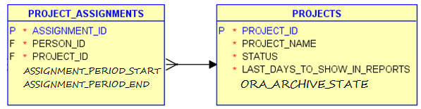
Tables that are defined as ROW ARCHIVAL have the hidden column ORA_ARCHIVE_STATE. By default, when we select from such tables a hidden predicate is added automatically: ORA_ARCHIVE_STATE = ‘0’.
As shown in Write Less with More – Part 3:

drop table projects cascade constraints;
create table projects (
       project_id integer not null constraint projects_pk primary key,
       project_name varchar2(100) not null,
       status number(1) not null,
       last_days_to_show_in_reports integer not null
)
ROW ARCHIVAL;

insert into projects values (1,'Project A',1,2);
insert into projects values (2,'Project B',2,3);
insert into projects values (3,'Project C',1,4);
insert into projects values (4,'Project D',2,3);
commit;

> update projects set ORA_ARCHIVE_STATE='1' where project_id in (1,3);

2 rows updated.

> select * from projects; 

                                      LAST_DAYS_TO
PROJECT_ID PROJECT_NAME     STATUS SHOW_IN_REPORTS
---------- ------------ ---------- ---------------
         2 Project B             2               3
         4 Project D             2               3 

> select * from table(dbms_xplan.display_cursor());

PLAN_TABLE_OUTPUT
------------------------------------------------------------------------------------
SQL_ID  dcthaywgmzra7, child number 1
-------------------------------------
select * from projects

Plan hash value: 2188942312

------------------------------------------------------------------------------
| Id  | Operation         | Name     | Rows  | Bytes | Cost (%CPU)| Time     |
------------------------------------------------------------------------------
|   0 | SELECT STATEMENT  |          |       |       |     3 (100)|          |
|*  1 |  TABLE ACCESS FULL| PROJECTS |     4 |  8372 |     3   (0)| 00:00:01 |
------------------------------------------------------------------------------

Predicate Information (identified by operation id):
---------------------------------------------------

   1 - filter("PROJECTS"."ORA_ARCHIVE_STATE"='0')

But when does Oracle add this predicate?

In this case, it’s not during expansion:

var x clob
begin
  dbms_utility.expand_sql_text(
    input_sql_text => 'select * from projects',
    output_sql_text => :x);
end;
/

PL/SQL procedure successfully completed.

print x

SELECT "A1"."PROJECT_ID"                   "PROJECT_ID",
       "A1"."PROJECT_NAME"                 "PROJECT_NAME",
       "A1"."STATUS"                       "STATUS",
       "A1"."LAST_DAYS_TO_SHOW_IN_REPORTS" "LAST_DAYS_TO_SHOW_IN_REPORTS"
FROM   "DEMO5"."PROJECTS" "A1"

A 10053 trace shows that the predicate is not added by the Query Transformer either (which I think is a good thing, as the Transformer should not change the meaning of the query):

.
.
.
******************************************
----- Current SQL Statement for this session (sql_id=dcthaywgmzra7) -----
select * from projects
*******************************************
.
.
.
=====================================
SPD: BEGIN context at statement level
=====================================
Stmt: ******* UNPARSED QUERY IS *******
SELECT "PROJECTS"."PROJECT_ID" "PROJECT_ID","PROJECTS"."PROJECT_NAME" "PROJECT_NAME","PROJECTS"."STATUS" "STATUS","PROJECTS"."LAST_DAYS_TO_SHOW_IN_REPORTS" "LAST_DAYS_TO_SHOW_IN_REPORTS" FROM "DEMO5"."PROJECTS" "PROJECTS" WHERE "PROJECTS"."ORA_ARCHIVE_STATE"='0'
Objects referenced in the statement
  PROJECTS[PROJECTS] 113224, type = 1
Objects in the hash table
  Hash table Object 113224, type = 1, ownerid = 8465150763180795273:
    No Dynamic Sampling Directives for the object
Return code in qosdInitDirCtx: ENBLD
===================================
SPD: END context at statement level
===================================
Final query after transformations:******* UNPARSED QUERY IS *******
SELECT "PROJECTS"."PROJECT_ID" "PROJECT_ID","PROJECTS"."PROJECT_NAME" "PROJECT_NAME","PROJECTS"."STATUS" "STATUS","PROJECTS"."LAST_DAYS_TO_SHOW_IN_REPORTS" "LAST_DAYS_TO_SHOW_IN_REPORTS" FROM "DEMO5"."PROJECTS" "PROJECTS" WHERE "PROJECTS"."ORA_ARCHIVE_STATE"='0'
kkoqbc: optimizing query block SEL$1 (#0)
.
.
.

A 10046 trace file contains no indication for ORA_ARCHIVE_STATE at all.

Comparing 10053 trace files of the statement select * from projects between two executions – one with the default behavior where the predicate is added and the second with “alter session set ROW ARCHIVAL VISIBILITY = ALL” which returns all the records with no filtering on ORA_ARCHIVE_STATE – shows only one significant difference: under Compilation Environment Dump we see that ilm_filter = 0 in the former and ilm_filter = 1 in the latter.

So the predicate on ORA_ARCHIVE_STATE is probably added by neither the Parser nor the Query Transformer. I don’t know who does add it and when, but it seems that it is not done in the “standard” way Oracle usually do such things. Perhaps if it would have been done in the standard way, this bug (look at the “The Bad News” section) would not have happened.

Implementing Arc Relationships with Virtual Columns

Virtual columns were added in Oracle 11g Release 1. We can implement the same concept using views, but one of the advantages that I see in virtual columns is that we can define foreign key constraints on them. Well, we can define foreign key constraints on views as well, but only in DISABLE NOVALIDATE mode, which makes them a decoration rather than a data integrity protector. So to be more precise, we can define enabled foreign key constraints on virtual columns.

This post is about using virtual columns for implementing arc relationships.

In the following ERD, the arc represents the rule “each Entity Address must be owned by either a Person or a Company”:
arc
There are three common ways to implement this logical data model.

Multiple Tables

We can split the ENTITY_ADDRESS entity into two tables – say, PERSON_ADDRESSES and COMPANY_ADDRESSES. Disadvantages of this solution are that we need to maintain two (or more) tables and the code parts that manipulate them, although they are very similar. In addition, if later on we need to add another entity to the relationship (for example, Store, in addition to Person and Company) we will have to add another join table – STORE_ADDRESSES – and the relevant code.

A Single Table with Dedicated Columns

We can implement the ENTITY_ADDRESS entity as a single table – say, ENTITY_ADDRESSES – with a dedicated column for each referenced entity – PERSON_ID and COMPANY_ID (in addition to ADDRESS_ID) – and a check constraint to make sure one and only one of the columns PERSON_ID and COMPANY_ID is not null. The disadvantage of this solution is that we still need to maintain the dedicated columns and the code parts that manipulate them, although they are very similar. And if we need to add another entity to the relationship we will have to add another column to the table and to add the relevant code to manipulate the new column.

A Generic Table

We can implement the ENTITY_ADDRESS entity as a single table – say, ENTITY_ADDRESSES – with a generic column for the referenced entity and a column that stores the entity type to which the generic column references – e.g., ADDRESS_ID, OWNER_TYPE_ID, OWNER_ID. The disadvantage of this solution is that we cannot define foreign key constraints from ENTITY_ADDRESSES to the PEOPLE and COMPANIES tables.

Using Virtual Columns

I’d like to suggest another solution, that, using virtual columns, overcomes the above disadvantages.
This solution is based on the generic table one, but we’ll add also a virtual column for each referenced entity. The purpose of the virtual columns is just for enforcing the referential integrity, and the application should not be aware of them. Therefore, if another entity should be added afterwards, we will add another virtual column, but we will have no code changes to make.

Here it is:

> create table people (
>   id integer not null primary key,
>   first_name varchar2(30) not null,
>   last_name varchar2(30) not null
> );

Table created.

> create table companies (
>   id integer not null primary key,
>   name varchar2(100) not null,
>   number_of_employees integer,
>   description varchar2(1000)
> );

Table created.

> create table addresses (
>   id integer not null primary key,
>   street varchar2(30),
>   house_number varchar2(10),
>   city varchar2(30),
>   country varchar2(30)
> );

Table created.
> create table entity_addresses (
>   address_id integer not null references addresses,
>   owner_type_id char(1) not null check (owner_type_id in ('P','C')),
>   owner_id integer not null,
>   --
>   primary key (owner_id,owner_type_id,address_id),
>   --
>   person_id generated always as (decode(owner_type_id,'P',owner_id)) virtual
>     constraint address_fk_people references people,
>   company_id generated always as (decode(owner_type_id,'C',owner_id)) virtual
>     constraint address_fk_companies references companies
> );

Table created. 
> insert into people (id,first_name,last_name) values (1,'John','Doe');

1 row created.

> insert into companies (id,name) values (101,'DB Oriented');

1 row created.

> insert into addresses (id,street,city,country) values (1,'Dekel','Zurit','Israel');

1 row created.

> insert into entity_addresses (address_id,owner_type_id,owner_id) 
> values (1,'P',1);

1 row created.

> insert into entity_addresses (address_id,owner_type_id,owner_id) 
> values (1,'P',101);
insert into entity_addresses (address_id,owner_type_id,owner_id) values (1,'P',101)
*
ERROR at line 1:
ORA-02291: integrity constraint (DEMO5.ADDRESS_FK_PEOPLE) violated - parent key not found


> insert into entity_addresses (address_id,owner_type_id,owner_id) 
> values (1,'C',1);
insert into entity_addresses (address_id,owner_type_id,owner_id) values (1,'C',1)
*
ERROR at line 1:
ORA-02291: integrity constraint (DEMO5.ADDRESS_FK_COMPANIES) violated - parent key not found


> insert into entity_addresses (address_id,owner_type_id,owner_id) 
> values (1,'C',101);

1 row created.

Hiding the Virtual Columns

Since the virtual columns in this solution are just for enforcing the referential integrity, I prefer to hide them, so adding new entities to the arc (or removing entities from it) will be transparent to the application.

Invisible Columns

In Oracle 12c we can do it by making these columns invisible.

> alter table entity_addresses modify (
>   person_id invisible,
>   company_id invisible
> );

Table altered.

> select * from entity_addresses;

ADDRESS_ID OWN   OWNER_ID
---------- --- ----------
         1 P            1
         1 C          101

Editioning Views

Being an Edition-Based Redefinition (EBR) evangelist, my application code never refers to tables. Each table is covered by an editioning view, and the application code refers only to views. This practice enables to hide the virtual columns very easily, simply by not including them in the editioning view:

> create editioning view entity_addresses_v as
>   select address_id,
>          owner_type_id,
>          owner_id
>   from entity_addresses;

View created.

Unfortunately, EBR is not widely used 🙁
You can, however, use the same idea in non-EBR environment, by creating a regular view rather than an editioning view, and refer to this view from the application code.

Write Less with More – Part 8 (PL/SQL in the WITH Clause)

This post is part 8 of the Write Less with More series of blog posts, focusing on new features of Oracle 12c that allow us developers to write less than in previous versions in order to achieve the same functionality. Each part is dedicated for one new feature that solves some common development task. For more details, including the setup of the examples used throughout the series and the list of development tasks that drive the series, please see part 1.

All the Series Parts

Part 1 – write less configuration with SQL*Loader Express Mode
Part 2 – write less application code with Identity Columns
Part 3 – write less application code with In-Database Archiving
Part 4 – write less application code with Temporal Validity
Part 5 – write less code in SQL with Row Limiting
Part 6 – write less “inappropriately located” code with SELECT FROM Package-Level Collection Types
Part 7 – write less code in SQL with Lateral Inline Views
Part 8 – write less “inappropriately located” code with PL/SQL in the WITH Clause

Task #8

todo8

We can write a small function – let’s call it is_date – that gets a string input and checks whether it represents a valid date or not, and then we can call the function from the SELECT statement:

select * from people where is_date(general_info) = 1;

The big question is where to locate the function.

A Pre-12c Solution

So where to locate the function? Before 12c we had only one choice: creating is_date as a stored function (either in a package or standalone), whose scope is the entire schema:

> create or replace function is_date(i_info in varchar2) return number as
      l_date date;
  begin
      if i_info is null then
          return 0;
      else
          l_date := to_date(i_info, 'dd/mm/yyyy');
          return 1;
      end if;
  exception
      when others then
          return 0;
  end is_date;
  /

Function created.

> select p.* from people p where is_date(p.general_info) = 1;

 PERSON_ID FIRST_NAME LAST_NAME       GENERAL_INFO
---------- ---------- --------------- --------------------
       102 Paul       McCartney       18/6/1942
       202 Ella       Fitzgerald      15/6/1996
       203 Etta       James           20/1/2012

But if is_date is used only in the context of this query, storing it and exposing it to the entire schema is quite inappropriate.

A 12c Solution

Oracle 12c offers a better option. The WITH clause can now include not only subquery factoring but also PL/SQL declarations of functions that can be used in the query (and procedures that can be used in those functions). This allows for embedding ad-hoc functions, that are relevant only for a specific SQL statement, in the statement itself. In our case:

> with 
    function is_date(i_info in varchar2) return number
    as
      l_date date;
    begin
      if i_info is null then
        return 0;
      else
        l_date := to_date(i_info, 'dd/mm/yyyy');
        return 1;
      end if;
    exception
      when others then
        return 0;
    end is_date;
  select p.* 
  from people p
  where is_date(p.general_info) = 1
  /
  
 PERSON_ID FIRST_NAME LAST_NAME       GENERAL_INFO
---------- ---------- --------------- --------------------
       102 Paul       McCartney       18/6/1942
       202 Ella       Fitzgerald      15/6/1996
       203 Etta       James           20/1/2012

Note: Subquery Factoring is the ability to define some query in the WITH clause, name it, and use this name in the FROM clause of the main query. Before 12c, Subquery Factoring was the only thing you could define in the WITH clause, so “Subquery Factoring” and “the WITH clause” became synonymous. This is probably the reason that now, in 12c, you can hear sometimes the inaccurate statement: “you can define PL/SQL functions in the Subquery Factoring clause”. The correct statement is that “you can define PL/SQL functions in the WITH clause, in addition to Subquery Factoring”.

If you want to learn about many more new features of Oracle 12c, you may be interested in one of my in-house training sessions, particularly the Oracle 12c New Features for Developers full-day seminar.

Recommended Reading: Neil Chandler has utilized this feature nicely in a recent post, by wrapping supplied stored procedures in WITH-level functions.

PL/SQL in SQL in PL/SQL

The PL/SQL language does not support yet the new syntax. If we try to use the previous example as a static SQL statement within a PL/SQL program unit, we’ll get a compilation error:

> create or replace procedure show_date_people as
  begin
      for l_rec in (
        with 
          function is_date(i_info in varchar2) return number as
            l_date date;
          begin
            if i_info is null then
              return 0;
            else
              l_date := to_date(i_info, 'dd/mm/yyyy');
              return 1;
            end if;
          exception
            when others then
              return 0;
          end;
        select p.*
        from   people p
        where  is_date(p.general_info) = 1
        )
      loop
          dbms_output.put_line(l_rec.id || ': ' || l_rec.first_name || ' ' || l_rec.last_name);
      end loop;
  end show_date_people;
  /
Warning: Procedure created with compilation errors.

> show err
Errors for PROCEDURE SHOW_DATE_PEOPLE:

LINE/COL ERROR
-------- -----------------------------------------------------------------
4/7      PL/SQL: SQL Statement ignored
5/18     PL/SQL: ORA-00905: missing keyword
6/22     PLS-00103: Encountered the symbol ";" when expecting one of the
         following:
         loop

We can overcome this limitation by using dynamic SQL instead of static SQL:

> create or replace procedure show_date_people as
      l_rc         sys_refcursor;
      l_id         people.person_id%type;
      l_first_name people.first_name%type;
      l_last_name  people.last_name%type;
  begin
      open l_rc for q''
        with 
          function is_date(i_info in varchar2) return number as
            l_date date;
          begin
            if i_info is null then
              return 0;
            else
              l_date := to_date(i_info, 'dd/mm/yyyy');
              return 1;
            end if;
          exception
            when others then
              return 0;
          end;
        select p.person_id,p.first_name,p.last_name
        from   people p
        where  is_date(p.general_info) = 1'';
      loop
          fetch l_rc
              into l_id,
                   l_first_name,
                   l_last_name;
          exit when l_rc%notfound;
          dbms_output.put_line(l_id || ': ' || l_first_name || ' ' || l_last_name);
      end loop;
      close l_rc;
  end show_date_people;
  /

Procedure created.

> exec show_date_people
102: Paul McCartney
202: Ella Fitzgerald
203: Etta James

PL/SQL procedure successfully completed.

Subqueries

If we use the new syntax in a subquery, and the top-level statement itself is not a SELECT with PL/SQL declarations, it will not work…

> select * from (
    with
      function is_date(i_info in varchar2) return number
      as
        l_date date;
      begin
        if i_info is null then
          return 0;
        else
          l_date := to_date(i_info, 'dd/mm/yyyy');
          return 1;
        end if;
      exception
        when others then
          return 0;
      end is_date;
    select p.*
    from people p
    where is_date(p.general_info) = 1
  )
  /
  with
  *
ERROR at line 2:
ORA-32034: unsupported use of WITH clause

unless… we add the WITH_PLSQL hint:

> select /*+ with_plsql */ * from (
    with
      function is_date(i_info in varchar2) return number
      as
        l_date date;
      begin
        if i_info is null then
          return 0;
        else
          l_date := to_date(i_info, 'dd/mm/yyyy');
          return 1;
        end if;
      exception
        when others then
          return 0;
      end is_date;
    select p.*
    from people p
    where is_date(p.general_info) = 1
  )
  /

 PERSON_ID FIRST_NAME LAST_NAME       GENERAL_INFO
---------- ---------- --------------- --------------------
       102 Paul       McCartney       18/6/1942
       202 Ella       Fitzgerald      15/6/1996
       203 Etta       James           20/1/2012

Performance Considerations?

Many times when this new feature is discussed, it is presented as a “performance feature”. Indeed, the performance of a query may be improved if instead of calling a stored function it calls an embedded function, since less context switches between the SQL engine and the PL/SQL engine are needed. However, in my opinion, the real strength of this feature is the ability to locate code in the most appropriate location. If a function is needed only in the context of a specific query, then the appropriate location to define this function is in the query itself, rather than littering the schema with a stored function. On the other hand side, if a function is useful for many different queries, then its appropriate location is in the schema level, so it can be defined once and reused by the various queries. In this case, embedding the function implementation in all the queries may have the advantage of performance improvement, but it also has the big disadvantage of code duplication.
If we need to improve the performance of such queries, then, before duplicating the code, we should consider other alternatives – such as scalar subquery cache or the UDF pragma.

Recommended Reading: Martin Widlake has recently wrote a couple of posts about the UDF pragma, including an example for a performance comparison between native SQL, traditional PL/SQL and PL/SQL with the UDF pragma, and an empirical analysis of UDF limitations.

Conclusion

We saw in this part of the Write Less with More series that PL/SQL in the WITH Clause allows us to write less “inappropriately located” code.
I hope you enjoyed the series. This was the last part of it.

Write Less with More – Part 7 (Lateral Inline Views)

This post is part 7 of the Write Less with More series of blog posts, focusing on new features of Oracle 12c that allow us developers to write less than in previous versions in order to achieve the same functionality. Each part is dedicated for one new feature that solves some common development task. For more details, including the setup of the examples used throughout the series and the list of development tasks that drive the series, please see part 1.

All the Series Parts

Published

Part 1 – write less configuration with SQL*Loader Express Mode
Part 2 – write less application code with Identity Columns
Part 3 – write less application code with In-Database Archiving
Part 4 – write less application code with Temporal Validity
Part 5 – write less code in SQL with Row Limiting
Part 6 – write less “inappropriately located” code with SELECT FROM Package-Level Collection Types
Part 7 – write less code in SQL with Lateral Inline Views
Part 8 – write less “inappropriately located” code with PL/SQL in the WITH Clause

Task #7

todo7

At this point, after using In-Database Archiving in part 3 and Temporal Validity in part 4, this is how the PROJECTS and PROJECT_ASSIGNMENTS tables look like:
ERD part 7
Assuming today is November 13th 2015, and assuming this is the content of the PROJECTS table:

> select project_id,
         project_name,
         last_days_to_show_in_reports
  from projects;

PROJECT_ID PROJECT_NA LAST_DAYS_TO_SHOW_IN_REPORTS
---------- ---------- ----------------------------
         1 Project A                             2
         2 Project B                             3
         3 Project C                             4

then the output of the query that we need to write should looks like this:

> select...

PROJECT_NAME DAY        NUM_OF_ASSIGNMENTS
------------ ---------- ------------------
Project A    13/11/2015                  3
Project A    12/11/2015                  3

Project B    13/11/2015                  2
Project B    12/11/2015                  4
Project B    11/11/2015                  5

Project C    13/11/2015                  1
Project C    12/11/2015                  0
Project C    11/11/2015                  0
Project C    10/11/2015                  1

Since LAST_DAYS_TO_SHOW_IN_REPORTS of Project A is 2, the query should return 2 rows for this project – for today and for yesterday.
LAST_DAYS_TO_SHOW_IN_REPORTS of Project B is 3, so the query should return 3 rows for this project – for today, for yestrday and for 2 days ago.
Similarly, the query should return 4 rows for project C, since LAST_DAYS_TO_SHOW_IN_REPORTS of this project is 4.

If you want to learn about many more new features of Oracle 12c, you may be interested in one of my in-house training sessions, particularly the Oracle 12c New Features for Developers full-day seminar.

NUM_OF_ASSIGNMENTS in each row is calculated simply as the number of rows in PROJECT_ASSIGNMENTS for the relevant project and day. Note that even if there are no assignments for specific project and day, the query should still return a row (with NUM_OF_ASSIGNMENTS=0), as you can see in the example in Project C at 11/11/2015 and 12/11/2015.

Generating the Last N Days

Let’s first see how to generate the last N days; for example, the last 4 days:

> select trunc(sysdate) + 1 - level day
  from dual
  connect by level <= 4;

DAY
----------
13/11/2015
12/11/2015
11/11/2015
10/11/2015

The Solution for a Fixed Number of Days

So if we were required to get the last 4 days (exactly 4) for each project, we would simply do a cartesian product between PROJECTS and an inline view with the previous query:

> break on project_name skip 1 dup

> select p.project_name,
         d.day
  from   projects p,
         (select trunc(sysdate) + 1 - level day
          from   dual
          connect by level <= 4) d
  order  by project_name,
            day desc;

PROJECT_NAME DAY
------------ ----------
Project A    13/11/2015
Project A    12/11/2015
Project A    11/11/2015
Project A    10/11/2015

Project B    13/11/2015
Project B    12/11/2015
Project B    11/11/2015
Project B    10/11/2015

Project C    13/11/2015
Project C    12/11/2015
Project C    11/11/2015
Project C    10/11/2015

and then we would add NUM_OF_ASSIGNMENTS.

A Pre-12c Solution

But the requirement here is to have a different number of days per project.
One option is to find the maximum possible number of days, generate this number of days for each project, and then filter out the excess records:

> select p.project_name,
         d.day
  from   projects p,
         (select level row_num,
                 trunc(sysdate) + 1 - level day
          from   dual
          connect by level <=
            (select max(last_days_to_show_in_reports) from projects)
         ) d
  where d.row_num <= p.last_days_to_show_in_reports
  order by project_name,
           day desc;

PROJECT_NAME DAY
------------ ----------
Project A    13/11/2015
Project A    12/11/2015

Project B    13/11/2015
Project B    12/11/2015
Project B    11/11/2015

Project C    13/11/2015
Project C    12/11/2015
Project C    11/11/2015
Project C    10/11/2015

But I don’t really like this solution. First, because it requires accessing PROJECTS twice. Second, because of the excess processing.
Another option is using Collection Unnesting:

> select p.project_name,
         d.column_value day
  from   projects p,
         table(
           cast(
	     multiset (
	       select trunc(sysdate) + 1 - level
               from   dual
               connect by level <= p.last_days_to_show_in_reports
	     )
           as sys.odcidatelist)
          ) d
  order  by project_name,
            day desc;

PROJECT_NAME DAY
------------ ----------
Project A    13/11/2015
Project A    12/11/2015

Project B    13/11/2015
Project B    12/11/2015
Project B    11/11/2015

Project C    13/11/2015
Project C    12/11/2015
Project C    11/11/2015
Project C    10/11/2015

This option addresses both issues that I dislike in the first option, but it is quite cumbersome, and if you don’t have an object type that matches the result of the MULTISET operator (I used sys.odcidatelist in the example) you need to create one.

A 12c Solution

In Oracle 12c an inline view can be defined as LATERAL. This allows the inline view to refer to other tables that appear to its left in the FROM clause. Which is exactly what we need here:

> select p.project_name,
         d.day
  from   projects p,
         LATERAL (select trunc(sysdate) + 1 - level day
                  from   dual
                  connect by level <= p.last_days_to_show_in_reports)  d
  order by project_name,
           day;

PROJECT_NAME DAY
------------ ----------
Project A    13/11/2015
Project A    12/11/2015

Project B    13/11/2015
Project B    12/11/2015
Project B    11/11/2015

Project C    13/11/2015
Project C    12/11/2015
Project C    11/11/2015
Project C    10/11/2015

Note: lateral inline views have been used internally by the optimizer in 11g, and could even be used by the end user in some undocumented and unsupported way.

Just to complete the solution, we need to add NUM_OF_ASSIGNMENTS to the result. For example, using outer join:

> select pd.project_name,
         pd.day,
         count(a.project_id) num_of_assignments
  from   (select p.project_id,
                 p.project_name,
                 d.day
          from   projects p,
                 lateral (select trunc(sysdate) + 1 - level day
                          from   dual
                          connect by level <= p.last_days_to_show_in_reports)  d) pd,
         project_assignments a
  where  nvl(a.assignment_period_start(+), date '0001-01-01') <= pd.day
  and    pd.day < nvl(a.assignment_period_end(+), date '9999-12-31')
  and    a.project_id(+) = pd.project_id
  group  by pd.project_name,
            pd.day
  order  by project_name,
            day;

PROJECT_NAME DAY        NUM_OF_ASSIGNMENTS
------------ ---------- ------------------
Project A    13/11/2015                  3
Project A    12/11/2015                  3

Project B    13/11/2015                  2
Project B    12/11/2015                  4
Project B    11/11/2015                  5

Project C    13/11/2015                  1
Project C    12/11/2015                  0
Project C    11/11/2015                  0
Project C    10/11/2015                  1

Another Example

My first post about an Oracle 12c feature was in 2013, when 12c has just been released. It was about Lateral Inline Views, and you can see there another example for using this feature.

Conclusion

We saw in this part of the Write Less with More series that Lateral Inline Views allow us to write less code in SQL.
The next post will be about another new Oracle 12c feature – PL/SQL in the WITH Clause.

Write Less with More – Part 6 (SELECT FROM Package-Level Collection Types)

This post is part 6 of the Write Less with More series of blog posts, focusing on new features of Oracle 12c that allow us developers to write less than in previous versions in order to achieve the same functionality. Each part is dedicated for one new feature that solves some common development task. For more details, including the setup of the examples used throughout the series and the list of development tasks that drive the series, please see part 1.

All the Series Parts

Published

Part 1 – write less configuration with SQL*Loader Express Mode
Part 2 – write less application code with Identity Columns
Part 3 – write less application code with In-Database Archiving
Part 4 – write less application code with Temporal Validity
Part 5 – write less code in SQL with Row Limiting
Part 6 – write less “inappropriately located” code with SELECT FROM Package-Level Collection Types
Part 7 – write less code in SQL with Lateral Inline Views
Part 8 – write less “inappropriately located” code with PL/SQL in the WITH Clause

Task #6

todo6

We need to write a stored procedure that gets a collection parameter of “project updates”, each one with PROJECT_ID, UPDATE_TIME and STATUS, and updates the PROJECTS table with the latest status of each project.
For example, the input parameter may look like this:

PROJECT ID UPDATE TIME STATUS
1 10:00 2
1 14:00 3
2 09:00 1
3 09:00 4
2 08:00 3
3 08:00 2
2 10:00 2

The highlighted lines are the lines we are interested in – the latest one for each project.
For project_id 1 the line with update_time 14:00 is the latest, so we need to update its status to 3.
For project_id 2 the line with update_time 10:00 is the latest, so we need to update its status to 2.
For project_id 3 the line with update_time 09:00 is the latest, so we need to update its status to 4.
The input parameter in this example does not contain information about other projects, so only the projects with PROJECT_ID 1, 2 and 3 should be updated.

Let’s start with the API. A nice solution would be to define the procedure and the necessary types in one package, like this:

  create or replace package projects_dl as 

    type proj_update_t is record(
      project_id  projects.project_id%type,
      update_time date,
      status      projects.status%type);

    type proj_update_tt is table of proj_update_t;

    procedure update_status(
        i_proj_update_list in proj_update_tt 
    );

  end projects_dl;

And now to the implementation: we can do it procedurally, but take a look at the input parameter – it looks like a table that we need to find some rows in it. It will be much nicer to use SQL and treat the collection parameter as a table.
Let’s start with a SQL query that uses the TABLE expression to un-nest the collection and finds the latest status for each project:

If you want to learn about many more new features of Oracle 12c, you may be interested in one of my in-house training sessions, particularly the Oracle 12c New Features for Developers full-day seminar.


select project_id,
       max(status) keep(dense_rank last order by update_time) latest_status
from table(i_proj_update_list)
group by project_id;

Note: I used here the LAST function in order to sort each group by one column (UPDATE_TIME) and get the value from another column (STATUS). If you want to learn more about this function (and its twin – the FIRST function), I wrote about it here.

Now we can use this query as the driving result set for a MERGE statement that updates the PROJECTS table:

      merge into projects p
      using ( select project_id,
                     max(status) keep(dense_rank last 
                       order by update_time) latest_status
              from table(i_proj_update_list)
              group by project_id ) i 
      on (p.project_id = i.project_id)
      when matched then
        update set p.status=i.latest_status;

Note: if you want to learn more about the MERGE statement, I wrote about it here.

And finally, we can use this MERGE statement as the body of our procedure:

  create or replace package body projects_dl as 

    procedure update_status(
      i_proj_update_list in proj_update_tt) is 
    begin 

      merge into projects p
      using ( select project_id,
                     max(status) keep(dense_rank last 
                       order by update_time) latest_status
              from table(i_proj_update_list)
              group by project_id ) i 
      on (p.project_id = i.project_id)
      when matched then
        update set p.status=i.latest_status;

    end update_status;
  end projects_dl;

This solution works nicely in Oracle 12c, but not in earlier versions. In 12c it is possible to select from package-level collection types. If we try to compile this package in 11g it will fail with the following error:

PL/SQL: SQL Statement ignored
ORA-22905: cannot access rows from a non-nested table item
PLS-00642: local collection types not allowed
           in SQL statements

A Pre-12c Solution

To achieve the same functionality in 11g we had to create the proj_update_t and proj_update_tt types in the schema level, rather than in the projects_dl package, although they are used only in the scope of this package:

CREATE OR REPLACE TYPE proj_update_t AS OBJECT (
    project_id  INTEGER,
    update_time DATE,
    status      INTEGER);
/

CREATE TYPE proj_update_tt AS TABLE OF proj_update_t;
/

CREATE OR REPLACE PACKAGE projects_dl AS 
    PROCEDURE update_status(
        i_proj_update_list IN proj_update_tt 
    );
END projects_dl;
/

Conclusion

We saw in this part of the Write Less with More series that “SELECT FROM Package-Level Collection Types” allows us to write less “inappropriately-located” code.
The next post will be about another new Oracle 12c feature – Lateral Inline Views.

Write Less with More – Part 5 (Row Limiting)

This post is part 5 of the Write Less with More series of blog posts, focusing on new features of Oracle 12c that allow us developers to write less than in previous versions in order to achieve the same functionality. Each part is dedicated for one new feature that solves some common development task. For more details, including the setup of the examples used throughout the series and the list of development tasks that drive the series, please see part 1.

All the Series Parts

Published

Part 1 – write less configuration with SQL*Loader Express Mode
Part 2 – write less application code with Identity Columns
Part 3 – write less application code with In-Database Archiving
Part 4 – write less application code with Temporal Validity
Part 5 – write less code in SQL with Row Limiting
Part 6 – write less “inappropriately located” code with SELECT FROM Package-Level Collection Types
Part 7 – write less code in SQL with Lateral Inline Views
Part 8 – write less “inappropriately located” code with PL/SQL in the WITH Clause

Task #5

todo5

Pagination is the ability to retrieve an ordered result set one “page” at a time; for example, getting the first 20 records in one query execution, getting the second page (records 21-40) in another execution, or even jumping to page 9 and getting records 161-180 in a third query execution.

A Pre-12c Solution

Before 12c we can implement pagination using inline views and the ROWNUM pseudo column (or analytic functions like ROW_NUMBER), and the result is quite cumbersome. Let’s see such a solution:

We start with the complete result set, with no pagination:

select project_id,
       person_id,
       assignment_id,
       assignment_period_start,
       assignment_period_end
from project_assignments
order by project_id,person_id;

PROJECT_ID  PERSON_ID ASSIGNMENT_ID ASSIGNMENT ASSIGNMENT
---------- ---------- ------------- ---------- ----------
         1        101            39 28/09/2015 30/09/2015
         1        101            38 22/09/2015 24/09/2015
         1        101            37 16/09/2015 18/09/2015
         1        101            40 04/10/2015 06/10/2015
         1        101            41 10/10/2015 12/10/2015
         1        102            44 06/10/2015 08/10/2015
         1        102            43 28/09/2015 30/09/2015
         1        102            42 20/09/2015 22/09/2015
         1        102            45 14/10/2015 16/10/2015
         1        102            46 22/10/2015 24/10/2015
         1        103            47            03/10/2015
         2        101            48 27/09/2015 30/09/2015
         2        102            49 27/09/2015 30/09/2015
         2        103            50 28/09/2015 30/09/2015
         2        104            51 28/09/2015 30/09/2015
         2        201            52 29/09/2015 30/09/2015
         3        101            53 26/09/2015 27/09/2015
         3        102            54 29/09/2015

18 rows selected.

If we want to get only the top 8 records, we can put the previous query in an inline view, and add a condition on ROWNUM:

select x.*
from (
  select project_id,
         person_id,
         assignment_id,
         assignment_period_start,
         assignment_period_end
  from project_assignments
  order by project_id,person_id
) x
where rownum <= 8;

PROJECT_ID  PERSON_ID ASSIGNMENT_ID ASSIGNMENT ASSIGNMENT
---------- ---------- ------------- ---------- ----------
         1        101            37 16/09/2015 18/09/2015
         1        101            38 22/09/2015 24/09/2015
         1        101            39 28/09/2015 30/09/2015
         1        101            40 04/10/2015 06/10/2015
         1        101            41 10/10/2015 12/10/2015
         1        102            42 20/09/2015 22/09/2015
         1        102            43 28/09/2015 30/09/2015
         1        102            44 06/10/2015 08/10/2015

8 rows selected.

If we want to get only records 5-8 (or, in other words, the second page where each page contains 4 records), we’ll add yet one more inline view:

select project_id,
       person_id,
       assignment_id,
       assignment_period_start,
       assignment_period_end 
from (
  select x.*
         ,rownum row_num 
  from (
    select project_id,
           person_id,
           assignment_id,
           assignment_period_start,
           assignment_period_end
    from project_assignments
    order by project_id,person_id
  ) x
  where rownum <= 8
)
where row_num > 4;

PROJECT_ID  PERSON_ID ASSIGNMENT_ID ASSIGNMENT ASSIGNMENT
---------- ---------- ------------- ---------- ----------
         1        101            41 10/10/2015 12/10/2015
         1        102            42 20/09/2015 22/09/2015
         1        102            43 28/09/2015 30/09/2015
         1        102            44 06/10/2015 08/10/2015

4 rows selected.

A 12c Solution

The Row Limiting Clause

In Oracle 12c this can be achieved using the new Row Limiting clause, which can be added to the end of SELECT statements. The size of the page is defined by either an absolute number of records or a specific percent of records out of the complete result set. You can define whether the page starts from the first record of the original result set or from some offset. It can also be defined how to treat “ties” (i.e., when several records with the same value are on the borders of the page).

If you want to learn about many more new features of Oracle 12c, you may be interested in one of my in-house training sessions, particularly the Oracle 12c New Features for Developers full-day seminar.

Top N Queries

To get only the first 4 rows:

select project_id,
       person_id,
       assignment_id,
       assignment_period_start,
       assignment_period_end
from project_assignments
order by project_id,person_id
FETCH FIRST 4 ROWS ONLY;

PROJECT_ID  PERSON_ID ASSIGNMENT_ID ASSIGNMENT ASSIGNMENT
---------- ---------- ------------- ---------- ----------
         1        101            37 16/09/2015 18/09/2015
         1        101            38 22/09/2015 24/09/2015
         1        101            39 28/09/2015 30/09/2015
         1        101            40 04/10/2015 06/10/2015

4 rows selected.

Note: the Row Limiting syntax is quite liberal. Wherever I use the ROWS keyword you can use either ROW or ROWS. Wherever I use FIRST or NEXT you can use either FIRST or NEXT.

Handling Ties

Take a look at the complete ordered result set above (the one that returned all the 18 rows of the table). You can see that the first 5 records have the same PROJET_ID (1) and PERSON_ID (101). It means that the previous query – that returned the first 4 rows – is not deterministic. It may return different 4 rows (out of 5) in different executions, because there is a tie between these 5 rows. The clause ORDER BY PROJECT_ID, PERSON_ID dictates that this set of 5 rows will be returned first, but it does not dictate the order within this set.
If we want to get a deterministic result, we can replace the keyword ONLY with WITH TIES:

select project_id,
       person_id,
       assignment_id,
       assignment_period_start,
       assignment_period_end
from project_assignments
order by project_id,person_id
FETCH FIRST 4 ROWS WITH TIES;

PROJECT_ID  PERSON_ID ASSIGNMENT_ID ASSIGNMENT ASSIGNMENT
---------- ---------- ------------- ---------- ----------
         1        101            37 16/09/2015 18/09/2015
         1        101            38 22/09/2015 24/09/2015
         1        101            39 28/09/2015 30/09/2015
         1        101            40 04/10/2015 06/10/2015
         1        101            41 10/10/2015 12/10/2015

5 rows selected.

FETCH FIRST 4 ROWS WITH TIES means that we get the first 4 rows, and all the successive rows that have the same values in the “ORDER BY” columns as the 4th record.

Top Percentage

We can ask for a specific percentage of the rows rather than a specific number of rows:

select project_id,
       person_id,
       assignment_id,
       assignment_period_start,
       assignment_period_end
from project_assignments
order by project_id,person_id
FETCH FIRST 50 PERCENT ROWS ONLY;

PROJECT_ID  PERSON_ID ASSIGNMENT_ID ASSIGNMENT ASSIGNMENT
---------- ---------- ------------- ---------- ----------
         1        101            39 28/09/2015 30/09/2015
         1        101            38 22/09/2015 24/09/2015
         1        101            37 16/09/2015 18/09/2015
         1        101            40 04/10/2015 06/10/2015
         1        101            41 10/10/2015 12/10/2015
         1        102            44 06/10/2015 08/10/2015
         1        102            43 28/09/2015 30/09/2015
         1        102            42 20/09/2015 22/09/2015
         1        102            45 14/10/2015 16/10/2015

9 rows selected.

Once again, this is not a deterministic result. To make it deterministic we use WITH TIES instead of ONLY, just as in the previous section:

select project_id,
       person_id,
       assignment_id,
       assignment_period_start,
       assignment_period_end
from project_assignments
order by project_id,person_id
FETCH FIRST 50 PERCENT ROWS WITH TIES;

PROJECT_ID  PERSON_ID ASSIGNMENT_ID ASSIGNMENT ASSIGNMENT
---------- ---------- ------------- ---------- ----------
         1        101            39 28/09/2015 30/09/2015
         1        101            38 22/09/2015 24/09/2015
         1        101            37 16/09/2015 18/09/2015
         1        101            40 04/10/2015 06/10/2015
         1        101            41 10/10/2015 12/10/2015
         1        102            44 06/10/2015 08/10/2015
         1        102            43 28/09/2015 30/09/2015
         1        102            42 20/09/2015 22/09/2015
         1        102            45 14/10/2015 16/10/2015
         1        102            46 22/10/2015 24/10/2015

10 rows selected.

Note that we got 10 rows, which is more than the requested 50%, because the 10th row has the same PROJECT_ID and PERSON_ID as the 9th row.

Performance Considerations

Note: The percentage option means that Oracle has to count first the total number of records in the underlying result set. This can consume significant resources and time for large data sets.

Recommended Reading: Franck Patchot has recently compared (in its excellent blog) the execution plans of three alternatives of Top N queries: using ROWNUM, using ROW_NUMBER and 12c Row Limiting.

Paging

To get only the 4 rows that follow the first 4 rows (i.e., rows 5-8), we add the OFFSET clause:

select project_id,
       person_id,
       assignment_id,
       assignment_period_start,
       assignment_period_end
from project_assignments
order by project_id,person_id
OFFSET 4 ROWS
FETCH NEXT 4 ROWS ONLY;

PROJECT_ID  PERSON_ID ASSIGNMENT_ID ASSIGNMENT ASSIGNMENT
---------- ---------- ------------- ---------- ----------
         1        101            41 10/10/2015 12/10/2015
         1        102            42 20/09/2015 22/09/2015
         1        102            43 28/09/2015 30/09/2015
         1        102            44 06/10/2015 08/10/2015

4 rows selected.

Behind the Scenes

Using the DBMS_UTILITY.EXPAND_SQL_TEXT procedure (yet another new feature of Oracle 12c), we can see that Oracle actually translates the new Row Limiting clause into conditions with analytic functions – ROW_NUMBER for the ONLY option and RANK for the WITH TIES option. Here are some examples:

var x clob
begin
  dbms_utility.expand_sql_text(
    input_sql_text => '
      select project_id,
             person_id,
             assignment_id,
             assignment_period_start,
             assignment_period_end
      from project_assignments
      order by project_id,person_id
      OFFSET 100 ROWS 
      FETCH NEXT 4 ROWS ONLY',
    output_sql_text => :x);
end;
/
 
print x

-- I formatted the output to make it more readable
SELECT "A1"."PROJECT_ID"              "PROJECT_ID",
       "A1"."PERSON_ID"               "PERSON_ID",
       "A1"."ASSIGNMENT_ID"           "ASSIGNMENT_ID",
       "A1"."ASSIGNMENT_PERIOD_START" "ASSIGNMENT_PERIOD_START",
       "A1"."ASSIGNMENT_PERIOD_END"   "ASSIGNMENT_PERIOD_END"
FROM   (SELECT "A2"."PROJECT_ID" "PROJECT_ID",
               "A2"."PERSON_ID" "PERSON_ID",
               "A2"."ASSIGNMENT_ID" "ASSIGNMENT_ID",
               "A2"."ASSIGNMENT_PERIOD_START" "ASSIGNMENT_PERIOD_START",
               "A2"."ASSIGNMENT_PERIOD_END" "ASSIGNMENT_PERIOD_END",
               "A2"."PROJECT_ID" "rowlimit_$_0",
               "A2"."PERSON_ID" "rowlimit_$_1",
               row_number() over(ORDER BY "A2"."PROJECT_ID", "A2"."PERSON_ID") "rowlimit_$$_rownumber"
        FROM   "DEMO5"."PROJECT_ASSIGNMENTS""A2") "A1"
WHERE  "A1"."rowlimit_$$_rownumber" <= CASE WHEN (100 >= 0) THEN floor(to_number(100)) ELSE 0 END + 4
AND    "A1"."rowlimit_$$_rownumber" > 100
ORDER  BY "A1"."rowlimit_$_0",
          "A1"."rowlimit_$_1"
begin
  dbms_utility.expand_sql_text(
    input_sql_text  => '
      select project_id,
             person_id,
             assignment_id,
             assignment_period_start,
             assignment_period_end
      from project_assignments
      order by project_id,person_id
      OFFSET 100 ROWS 
      FETCH NEXT 4 ROWS WITH TIES',
    output_sql_text => :x);
end;
/
 
print x

-- I formatted the output to make it more readable
SELECT "A1"."PROJECT_ID"              "PROJECT_ID",
       "A1"."PERSON_ID"               "PERSON_ID",
       "A1"."ASSIGNMENT_ID"           "ASSIGNMENT_ID",
       "A1"."ASSIGNMENT_PERIOD_START" "ASSIGNMENT_PERIOD_START",
       "A1"."ASSIGNMENT_PERIOD_END"   "ASSIGNMENT_PERIOD_END"
FROM   (SELECT "A2"."PROJECT_ID" "PROJECT_ID",
               "A2"."PERSON_ID" "PERSON_ID",
               "A2"."ASSIGNMENT_ID" "ASSIGNMENT_ID",
               "A2"."ASSIGNMENT_PERIOD_START" "ASSIGNMENT_PERIOD_START",
               "A2"."ASSIGNMENT_PERIOD_END" "ASSIGNMENT_PERIOD_END",
               "A2"."PROJECT_ID" "rowlimit_$_0",
               "A2"."PERSON_ID" "rowlimit_$_1",
               row_number() over(ORDER BY "A2"."PROJECT_ID", "A2"."PERSON_ID") "rowlimit_$$_rownumber",
               rank() over(ORDER BY "A2"."PROJECT_ID", "A2"."PERSON_ID") "rowlimit_$$_rank"
        FROM   "DEMO5"."PROJECT_ASSIGNMENTS" "A2") "A1"
WHERE  "A1"."rowlimit_$$_rank" <= CASE WHEN (100 >= 0) THEN floor(to_number(100)) ELSE 0 END + 4
AND    "A1"."rowlimit_$$_rownumber" > 100
ORDER  BY "A1"."rowlimit_$_0",
          "A1"."rowlimit_$_1"
begin
  dbms_utility.expand_sql_text(
    input_sql_text  => '
      select project_id,
             person_id,
             assignment_id,
             assignment_period_start,
             assignment_period_end
      from project_assignments
      order by project_id,person_id
      FETCH FIRST 10 percent ROWS only',
    output_sql_text => :x);
end;
/
 
print x
-- I formatted the output to make it more readable

SELECT "A1"."PROJECT_ID"              "PROJECT_ID",
       "A1"."PERSON_ID"               "PERSON_ID",
       "A1"."ASSIGNMENT_ID"           "ASSIGNMENT_ID",
       "A1"."ASSIGNMENT_PERIOD_START" "ASSIGNMENT_PERIOD_START",
       "A1"."ASSIGNMENT_PERIOD_END"   "ASSIGNMENT_PERIOD_END"
FROM   (SELECT "A2"."PROJECT_ID" "PROJECT_ID",
               "A2"."PERSON_ID" "PERSON_ID",
               "A2"."ASSIGNMENT_ID" "ASSIGNMENT_ID",
               "A2"."ASSIGNMENT_PERIOD_START" "ASSIGNMENT_PERIOD_START",
               "A2"."ASSIGNMENT_PERIOD_END" "ASSIGNMENT_PERIOD_END",
               "A2"."PROJECT_ID" "rowlimit_$_0",
               "A2"."PERSON_ID" "rowlimit_$_1",
               row_number() over(ORDER BY "A2"."PROJECT_ID", "A2"."PERSON_ID") "rowlimit_$$_rownumber",
               COUNT(*) over() "rowlimit_$$_total"
        FROM   "DEMO5"."PROJECT_ASSIGNMENTS" "A2") "A1"
WHERE  "A1"."rowlimit_$$_rownumber" <= ceil("A1"."rowlimit_$$_total" * 10 / 100)
ORDER  BY "A1"."rowlimit_$_0",
          "A1"."rowlimit_$_1"

Conclusion

We saw in this part of the Write Less with More series that Row Limiting allows us to write less code in SQL.
The next post will be about another new Oracle 12c feature – SELECT FROM Package-Level Collection Types.

Write Less with More – Part 4 (Temporal Validity)

This post is part 4 of the Write Less with More series of blog posts, focusing on new features of Oracle 12c that allow us developers to write less than in previous versions in order to achieve the same functionality. Each part is dedicated for one new feature that solves some common development task. For more details, including the setup of the examples used throughout the series and the list of development tasks that drive the series, please see part 1.

All the Series Parts

Published

Part 1 – write less configuration with SQL*Loader Express Mode
Part 2 – write less application code with Identity Columns
Part 3 – write less application code with In-Database Archiving
Part 4 – write less application code with Temporal Validity
Part 5 – write less code in SQL with Row Limiting
Part 6 – write less “inappropriately located” code with SELECT FROM Package-Level Collection Types
Part 7 – write less code in SQL with Lateral Inline Views
Part 8 – write less “inappropriately located” code with PL/SQL in the WITH Clause

Task #4

todo4

PROJECT_ASSIGNMENTS is too simplistic. At this point (after it was defined in part 1 and enhanced in Part 2) it only says which people are assigned to which projects, not when or for how long. Now we want to add this missing information.

A Pre-12c Solution

Before 12c we could add a pair of date/time columns to represent the active period boundaries, e.g. PERIOD_START and PERIOD_END:

alter table project_assignments add (
  period_start date,
  period_end   date
);

When dealing with time periods there are three important decisions to make:
One decision is how to represent periods that their start point or end point (or even both) are unlimited. I will use NULL for this.

I recommend reading Stew Ashton’s post about his preference of not using NULL to represent unlimited period boundaries. It doesn’t matter if you agree or not – reading about the reasons is the important part. Actually, I recommend reading everything Stew writes 🙂


Another decision is whether the period boundaries are inclusive or exclusive. I like to include the start point in the period and exclude the end point. In this way, if we want to assign someone to a project for the whole month of February 2015 (for example) we will use quite simple values:

insert into project_assignments (person_id,project_id,period_start,period_end)
values (101,1,date'2015-02-01',date'2015-03-01');

If I’d choose to include both the start point and the end point in the period, I would have to use a more complex value:

insert into project_assignments (person_id,project_id,period_start,period_end)
values (101,1,date'2015-02-01',timestamp'2015-02-28 23:59:59');

And a third decision is which data type to use for the start/end columns – DATE, TIMESTAMP or TIMESTAMP WITH TIME ZONE. This decision is derived from the functional requirements for period boundary granularity (and your data modeling standards, if you have any [I hope you do]).

After we added the columns to the table, we need to add conditions to all the relevant SQL statements in the application (or applications).
For example, if we want to get all the assignments that are active on a specific date:

select * from project_assignments a
where (a.period_start is null or a.period_start <= :my_date)
  and (a.period_end is null or a.period_end > :my_date);

And if we want to get all the assignments that are active sometime within a specific time range:

select * from project_assignments a
where (a.period_start is null or a.period_start < :my_end_date)
  and (a.period_end is null or a.period_end > :my_start_date);

A 12c Solution

Temporal Validity

In Oracle 12c a table can be defined with the PERIOD FOR clause, to associate it with one or more valid time dimensions. Each such dimension consists of a pair of date/time columns. These columns can be created either explicitly or implicitly. As a result, the data can become visible or invisible, based on statement- or session-level definitions.
In our case we can simply add a period called ASSIGNMENT_PERIOD to the table:
 

alter table project_assignments 
       add PERIOD FOR assignment_period;

This statement added two hidden TIMESTAMP WITH TIME ZONE columns – ASSIGNMENT_PERIOD_START and ASSIGNMENT_PERIOD_END – which can (and should) be set explicitly when records of PROJECT_ASSIGNMENTS are inserted and updated.
When we DESCRIBE the table, we see only the columns we explicitly defined:

> desc project_assignments
 Name                                         Null?    Type
 -------------------------------------------- -------- ----------------------
 ASSIGNMENT_ID                                NOT NULL NUMBER(38)
 PERSON_ID                                    NOT NULL NUMBER(38)
 PROJECT_ID                                   NOT NULL NUMBER(38)

But if we select from USER_TAB_COLS we discover the new columns – ASSIGNMENT_PERIOD_START and ASSIGNMENT_PERIOD_END (and one virtual column – ASSIGNMENT_PERIOD – that I will not discuss here):

> select column_name,data_type,nullable,hidden_column,virtual_column,user_generated
    from user_tab_cols
    where table_name = 'PROJECT_ASSIGNMENTS';

COLUMN_NAME                    DATA_TYPE                   NUL HIDDEN_CO VIRTUAL_C USER_GENE
------------------------------ --------------------------- --- --------- --------- ---------
ASSIGNMENT_ID                  NUMBER                      N   NO        NO        YES
PERSON_ID                      NUMBER                      N   NO        NO        YES
PROJECT_ID                     NUMBER                      N   NO        NO        YES
ASSIGNMENT_PERIOD_START        TIMESTAMP(6) WITH TIME ZONE Y   YES       NO        NO
ASSIGNMENT_PERIOD_END          TIMESTAMP(6) WITH TIME ZONE Y   YES       NO        NO
ASSIGNMENT_PERIOD              NUMBER                      Y   YES       YES       NO

Note: there is a major difference between the data dictionary views USER_TAB_COLUMNS and USER_TAB_COLS: while the former exposes only the explicitly defined columns, the latter includes also system-generated columns.

Update [17-Sep-2021] Connor McDonald shows how the period information is stored in the data dictionary – https://connor-mcdonald.com/2021/09/17/is-my-table-temporal/

In addition to the columns, Oracle also implicitly created a check constraint, to make sure the start time is always before the end time:

> select constraint_name,constraint_type,search_condition
  from user_constraints
  where table_name='PROJECT_ASSIGNMENTS'
    and constraint_name like 'ASSIGNMENT_PERIOD%';

CONSTRAINT_NAME                CON SEARCH_CONDITION
------------------------------ --- ------------------------------------------------------
ASSIGNMENT_PERIOD3366E0        C   ASSIGNMENT_PERIOD_START < ASSIGNMENT_PERIOD_END

Note that the condition is “less than” and not “less than or equal to”. The Temporal Validity feature uses the same rule I used in the pre-12c solution – the period includes the start time and excludes the end time.

Now, let’s fill the table with some data. We need to explicitly set values to the system-generated columns:

insert into project_assignments
    (person_id,
     project_id,
     assignment_period_start,
     assignment_period_end)
values
    (101,
     1,
     date'2015-09-16',
     date'2015-09-18');

I added some more records as a preparation for the next examples. This is the content of the table at this point:

> select person_id,
         project_id,
         assignment_period_start,
         assignment_period_end
  from   project_assignments
  order  by assignment_period_start,
            assignment_period_end;

                      PERIOD     PERIOD
 PERSON_ID PROJECT_ID START      END
---------- ---------- ---------- ----------
       101          1 16/09/2015 18/09/2015
       102          1 20/09/2015 22/09/2015
       101          1 22/09/2015 24/09/2015
       101          3 26/09/2015 27/09/2015
       101          2 27/09/2015 30/09/2015
       102          2 27/09/2015 30/09/2015
       101          1 28/09/2015 30/09/2015
       104          2 28/09/2015 30/09/2015
       103          2 28/09/2015 30/09/2015
       102          1 28/09/2015 30/09/2015
       201          2 29/09/2015 30/09/2015
       102          3 29/09/2015
       101          1 04/10/2015 06/10/2015
       102          1 06/10/2015 08/10/2015
       101          1 10/10/2015 12/10/2015
       102          1 14/10/2015 16/10/2015
       102          1 22/10/2015 24/10/2015
       103          1            03/10/2015

18 rows selected.

Nulls represent unlimited start time or end time.

Statement-Level Control

To get, in a specific statement, only records that are active on a specific date, we add the AS OF PERIOD clause.
For example, to get only the project assignments that are active today (when today is September 29th, 2015):

> select person_id,
         project_id,
         assignment_period_start,
         assignment_period_end
  from   project_assignments
  AS OF PERIOD FOR assignment_period SYSDATE;

                      PERIOD     PERIOD
 PERSON_ID PROJECT_ID START      END
---------- ---------- ---------- ----------
       101          1 28/09/2015 30/09/2015
       102          1 28/09/2015 30/09/2015
       103          1            03/10/2015
       101          2 27/09/2015 30/09/2015
       102          2 27/09/2015 30/09/2015
       103          2 28/09/2015 30/09/2015
       104          2 28/09/2015 30/09/2015
       201          2 29/09/2015 30/09/2015
       102          3 29/09/2015

9 rows selected.

Or to get only the project assignments that will be active on October 10th, 2015:

> select person_id,
         project_id,
         assignment_period_start,
         assignment_period_end
  from   project_assignments
  AS OF PERIOD FOR assignment_period date'2015-10-10';

                      PERIOD     PERIOD
 PERSON_ID PROJECT_ID START      END
---------- ---------- ---------- ----------
       101          1 10/10/2015 12/10/2015
       102          3 29/09/2015

If we want to get only records that are active in a specific time range, we use the VERSIONS PERIOD clause. For example:

> select person_id,
         project_id,
         assignment_period_start,
         assignment_period_end
  from   project_assignments
  VERSIONS PERIOD FOR assignment_period
    between date'2015-09-21' and date'2015-09-23';

                      PERIOD     PERIOD
 PERSON_ID PROJECT_ID START      END
---------- ---------- ---------- ----------
       101          1 22/09/2015 24/09/2015
       102          1 20/09/2015 22/09/2015
       103          1            03/10/2015

Session-Level Control

We can also filter non-active records out in the session-level, affecting all the statements without changing them. We do it by calling the procedure DBMS_FLASHBACK_ARCHIVE.ENABLE_AT_VALID_TIME. This procedure has 3 options.
The first option it to pass the value ‘CURRENT’ to the LEVEL parameter (the first parameter), which means that all the subsequent statements in the session will consider only records that are active (or valid) at the execution time, for all the tables that were defined with the PERIOD FOR clause.

> exec dbms_flashback_archive.enable_at_valid_time('CURRENT')

PL/SQL procedure successfully completed.

> select person_id,
         project_id,
         assignment_period_start,
         assignment_period_end
  from   project_assignments;

                      PERIOD     PERIOD
 PERSON_ID PROJECT_ID START      END
---------- ---------- ---------- ----------
       101          1 28/09/2015 30/09/2015
       102          1 28/09/2015 30/09/2015
       103          1            03/10/2015
       101          2 27/09/2015 30/09/2015
       102          2 27/09/2015 30/09/2015
       103          2 28/09/2015 30/09/2015
       104          2 28/09/2015 30/09/2015
       201          2 29/09/2015 30/09/2015
       102          3 29/09/2015

9 rows selected.

The second option is to pass the value ‘ASOF’ (read “as of”) to the LEVEL parameter. In this case we need to pass also a concrete timestamp value to the QUERY_TIME parameter (the second parameter).

> exec dbms_flashback_archive.enable_at_valid_time('ASOF',date'2015-10-10')

PL/SQL procedure successfully completed.

> select person_id,
         project_id,
         assignment_period_start,
         assignment_period_end
  from   project_assignments;

                      PERIOD     PERIOD
 PERSON_ID PROJECT_ID START      END
---------- ---------- ---------- ----------
       101          1 10/10/2015 12/10/2015
       102          3 29/09/2015

And the third option is to pass the value ‘ALL’ to the LEVEL parameter, which means no filtering occurs in subsequent statements.

> exec dbms_flashback_archive.enable_at_valid_time('ALL')

PL/SQL procedure successfully completed.

> select person_id,
         project_id,
         assignment_period_start,
         assignment_period_end
  from   project_assignments;

                      PERIOD     PERIOD
 PERSON_ID PROJECT_ID START      END
---------- ---------- ---------- ----------
       101          1 16/09/2015 18/09/2015
       101          1 22/09/2015 24/09/2015
       101          1 28/09/2015 30/09/2015
       101          1 04/10/2015 06/10/2015
       101          1 10/10/2015 12/10/2015
       102          1 20/09/2015 22/09/2015
       102          1 28/09/2015 30/09/2015
       102          1 06/10/2015 08/10/2015
       102          1 14/10/2015 16/10/2015
       102          1 22/10/2015 24/10/2015
       103          1            03/10/2015
       101          2 27/09/2015 30/09/2015
       102          2 27/09/2015 30/09/2015
       103          2 28/09/2015 30/09/2015
       104          2 28/09/2015 30/09/2015
       201          2 29/09/2015 30/09/2015
       101          3 26/09/2015 27/09/2015
       102          3 29/09/2015

18 rows selected.

Warning:
if the value you pass to the LEVEL parameter of dbms_flashback_archive.enable_at_valid_time is other than ‘CURRENT’, ‘ASOF’ or ‘ALL’, it will NOT change anything and the previous setting will still take effect.
The dangerous part is that the procedure does not throw any exception; it completes successfully (doing nothing).
And these 3 values are case-sensitive. Passing ‘current’ or ‘AsOf’, for example, will silently do nothing.

There are two sides to every coin

We’ve just seen that Temporal Validity adds hidden columns to tables and hidden predicates to SQL statements. This is cool, but also dangerous. When things are hidden, it is easy to forget them, but we shouldn’t. See what I’ve already written about that with regards to In-Database Archiving in part 3.

Conclusion

We saw in this part of the Write Less with More series that Temporal Validity allows us to write less application code.

The next post will be about another new Oracle 12c feature – Row Limiting.

When X+0 and X-0 are not the same

In the old days, when the Rule Based Optimizer (RBO) ruled, there was a very common technique to help the optimizer choose one plan over the other (if they had the same rank) by preventing the use of an index.

Look at the following query, where there are unique indexes on T1.ID and T2.ID and non-unique indexes on T1.A and T2.B:

select *
  from T1,T2
 where T1.ID = T2.ID
   and T1.A = :value1
   and T2.B = :value2;

One possible plan is to use nested loops, starting by accessing T1 via the index on A and then accessing T2 via the index on ID.
A second possible plan is to use nested loops, starting by accessing T2 via the index on B and then accessing T1 via the index on ID.

For the RBO these two plans were similar. If we wanted to convince the RBO to choose the second plan, a common trick was to prevent the use of the index on T1.A by adding “+0” to the condition:

select *
  from T1,T2
 where T1.ID = T2.ID
   and T1.A + 0 = :value1
   and T2.B = :value2;

What happens if we try using the same technique today, with the Cost Based Optimizer (CBO)?
Not that I recommend it!
It’s certainly not the way to influence the CBO, but I admit that I recently used it myself (it was in some weird constrained situation, please don’t ask…) and something surprised me. I’ll show you what in this post.

But first…
What is the cardinality of “column = some_value” (i.e., how many rows will return from this condition)? When the CBO doesn’t have histograms, its best guess is the number of rows in the table / the number of distinct values in the column.
And what is the cardinality of “some_function_of_column = some_value”? Without extended statistics or virtual columns, the CBO simply guesses that the cardinality is 1% of the table.
Keep this in mind.

I’ll start by crafting an example:

-- 10000 rows in T1
-- 5000 distinct values in A
-- A=0 in 5000 rows
create table t1 as 
  select rownum id,
         case when rownum<5000 then rownum else 0 end a, 
         lpad('x',100,'x') x
    from dual
 connect by level<=10000;

alter table t1 
  add constraint t1_pk primary key (id);

create index t1_i1 on t1 (a);

-- 1000 rows in T2
-- 21 distinct values in B
-- B=0 in 1 row only
create table t2 as 
  select rownum id,
         case when rownum<1000 then ceil(rownum/50) else 0 end b,
         lpad('x',10,'x') x 
    from dual 
 connect by level<=1000;

alter table t2 
  add constraint t2_pk primary key (id);

create index t2_i1 on t2 (b);

begin
  dbms_stats.gather_table_stats(user,'T1',method_opt =>'for all columns size 1',cascade => true);
  dbms_stats.gather_table_stats(user,'T2',method_opt =>'for all columns size 1',cascade => true);
end;
/

Note that I gathered statistics, but without histograms.

Now let’s run the following query:

> set autotrace on

> select *
    from T1,T2
   where T1.ID = T2.ID
     and T1.A = 0
     and T2.B = 0;

no rows selected

Execution Plan
----------------------------------------------------------
Plan hash value: 1001848667

---------------------------------------------------------------------------------------
| Id  | Operation                     | Name  | Rows  | Bytes | Cost (%CPU)| Time     |
---------------------------------------------------------------------------------------
|   0 | SELECT STATEMENT              |       |     2 |   252 |     3   (0)| 00:00:01 |
|   1 |  NESTED LOOPS                 |       |     2 |   252 |     3   (0)| 00:00:01 |
|   2 |   NESTED LOOPS                |       |     2 |   252 |     3   (0)| 00:00:01 |
|   3 |    TABLE ACCESS BY INDEX ROWID| T1    |     2 |   216 |     2   (0)| 00:00:01 |
|*  4 |     INDEX RANGE SCAN          | T1_I1 |     2 |       |     1   (0)| 00:00:01 |
|*  5 |    INDEX UNIQUE SCAN          | T2_PK |     1 |       |     0   (0)| 00:00:01 |
|*  6 |   TABLE ACCESS BY INDEX ROWID | T2    |     1 |    18 |     1   (0)| 00:00:01 |
---------------------------------------------------------------------------------------

Predicate Information (identified by operation id):
---------------------------------------------------
   4 - access("T1"."A"=0)
   5 - access("T1"."ID"="T2"."ID")
   6 - filter("T2"."B"=0)

Statistics
----------------------------------------------------------
          0  recursive calls
          0  db block gets
         99  consistent gets
          0  physical reads
          0  redo size
        646  bytes sent via SQL*Net to client
        513  bytes received via SQL*Net from client
          1  SQL*Net roundtrips to/from client
          0  sorts (memory)
          0  sorts (disk)
          0  rows processed

Without histograms the optimizer assumes uniform distribution, so the estimated cardinality of “T1.A=0” is 2 rows (=10000 rows in the table / 5000 distinct values in A), as we can see in the execution plan. And the estimated cardinality of “T2.B=0” is about 48 rows (=1000 rows in the table / 21 distinct values).
But we know that the data is skewed. The actual cardinality of “T1.A=0” is 5000 rows (there are 5000 rows out of 10000 with the value 0 in T1.A), and the actual cardinality of “T2.B=0” is 1 row. So it will be much better in this case to start the plan by accessing the index on T2.B.
The sensible way would be to gather histograms on the columns with the skewed data, to use the cardinality hint, or other “modern” approach. But what will happen if we use the old trick of preventing using the index on T1.A by adding “+0”? Let’s see:

> select *
    from T1,T2
   where T1.ID = T2.ID
     and T1.A + 0 = 0
     and T2.B = 0;

no rows selected

Execution Plan
----------------------------------------------------------
Plan hash value: 1837274416

--------------------------------------------------------------------------------------
| Id  | Operation                    | Name  | Rows  | Bytes | Cost (%CPU)| Time     |
--------------------------------------------------------------------------------------
|   0 | SELECT STATEMENT             |       |     2 |   252 |    49   (0)| 00:00:01 |
|   1 |  NESTED LOOPS                |       |     2 |   252 |    49   (0)| 00:00:01 |
|   2 |   NESTED LOOPS               |       |     2 |   252 |    49   (0)| 00:00:01 |
|*  3 |    TABLE ACCESS FULL         | T1    |     2 |   216 |    48   (0)| 00:00:01 |
|*  4 |    INDEX UNIQUE SCAN         | T2_PK |     1 |       |     0   (0)| 00:00:01 |
|*  5 |   TABLE ACCESS BY INDEX ROWID| T2    |     1 |    18 |     1   (0)| 00:00:01 |
--------------------------------------------------------------------------------------

Predicate Information (identified by operation id):
---------------------------------------------------
   3 - filter("T1"."A"+0=0)
   4 - access("T1"."ID"="T2"."ID")
   5 - filter("T2"."B"=0)

Statistics
----------------------------------------------------------
          0  recursive calls
          0  db block gets
        170  consistent gets
          0  physical reads
          0  redo size
        646  bytes sent via SQL*Net to client
        513  bytes received via SQL*Net from client
          1  SQL*Net roundtrips to/from client
          0  sorts (memory)
          0  sorts (disk)
          0  rows processed

Hurray! we succeeded to prevent the use of the index on T1.A. But, wait, the cardinality estimation was not changed – it is still 2. I would expect it to be 100 rows – 1% of 10000 – the usual guess of the CBO in case of “function_of_some_column = some_value”.
And because of this estimation, the plan still starts from T1, but this time with a full table scan (as we neutralized the index use). And this is a worse plan than the first one – note the 170 consistent gets compared to 99 before.

So the CBO is smart enough to realize that A+0 = A.

What about A-0 or A*1 ? Let’s try:

> select *
    from T1,T2
   where T1.ID = T2.ID
     and T1.A - 0 = 0
     and T2.B = 0;

no rows selected

Execution Plan
----------------------------------------------------------
Plan hash value: 1272512196

---------------------------------------------------------------------------------------
| Id  | Operation                     | Name  | Rows  | Bytes | Cost (%CPU)| Time     |
---------------------------------------------------------------------------------------
|   0 | SELECT STATEMENT              |       |    48 |  6048 |    50   (0)| 00:00:01 |
|   1 |  NESTED LOOPS                 |       |    48 |  6048 |    50   (0)| 00:00:01 |
|   2 |   NESTED LOOPS                |       |    48 |  6048 |    50   (0)| 00:00:01 |
|   3 |    TABLE ACCESS BY INDEX ROWID| T2    |    48 |   864 |     2   (0)| 00:00:01 |
|*  4 |     INDEX RANGE SCAN          | T2_I1 |    48 |       |     1   (0)| 00:00:01 |
|*  5 |    INDEX UNIQUE SCAN          | T1_PK |     1 |       |     0   (0)| 00:00:01 |
|*  6 |   TABLE ACCESS BY INDEX ROWID | T1    |     1 |   108 |     1   (0)| 00:00:01 |
---------------------------------------------------------------------------------------

Predicate Information (identified by operation id):
---------------------------------------------------
   4 - access("T2"."B"=0)
   5 - access("T1"."ID"="T2"."ID")
   6 - filter("T1"."A"-0=0)

Statistics
----------------------------------------------------------
          1  recursive calls
          0  db block gets
          6  consistent gets
          0  physical reads
          0  redo size
        646  bytes sent via SQL*Net to client
        513  bytes received via SQL*Net from client
          1  SQL*Net roundtrips to/from client
          0  sorts (memory)
          0  sorts (disk)
          0  rows processed

We changed “A+0” to “A-0″ and got a totally different execution plan! Unlike with A+0, the CBO does not realize that A-0=A. It treats A-0 just as any other function, and guesses that the cardinality of “A-0=0” is 1% of T1, which is 100 rows.

Remember that the example I used has no real significance. I just tried to mimic an old technique that was relevant for the RBO and is not appropriate for the CBO.

The important part is that the CBO gives a special treatment to COLUMN + 0 when it calculates cardinality. We can see it more explicitly from the following execution plans:

> select * from T1 where A = :val;

Execution Plan
----------------------------------------------------------
Plan hash value: 1429545322

-------------------------------------------------------------------------------------
| Id  | Operation                   | Name  | Rows  | Bytes | Cost (%CPU)| Time     |
-------------------------------------------------------------------------------------
|   0 | SELECT STATEMENT            |       |     2 |   216 |     2   (0)| 00:00:01 |
|   1 |  TABLE ACCESS BY INDEX ROWID| T1    |     2 |   216 |     2   (0)| 00:00:01 |
|*  2 |   INDEX RANGE SCAN          | T1_I1 |     2 |       |     1   (0)| 00:00:01 |
-------------------------------------------------------------------------------------

Predicate Information (identified by operation id):
---------------------------------------------------
   2 - access("A"=TO_NUMBER(:VAL))
> select * from T1 where A + 0 = :val;

Execution Plan
----------------------------------------------------------
Plan hash value: 3617692013

--------------------------------------------------------------------------
| Id  | Operation         | Name | Rows  | Bytes | Cost (%CPU)| Time     |
--------------------------------------------------------------------------
|   0 | SELECT STATEMENT  |      |     2 |   216 |    48   (0)| 00:00:01 |
|*  1 |  TABLE ACCESS FULL| T1   |     2 |   216 |    48   (0)| 00:00:01 |
--------------------------------------------------------------------------

Predicate Information (identified by operation id):
---------------------------------------------------
   1 - filter("A"+0=TO_NUMBER(:VAL))
> select * from T1 where A - 0 = :val;

Execution Plan
----------------------------------------------------------
Plan hash value: 3617692013

--------------------------------------------------------------------------
| Id  | Operation         | Name | Rows  | Bytes | Cost (%CPU)| Time     |
--------------------------------------------------------------------------
|   0 | SELECT STATEMENT  |      |   100 | 10800 |    48   (0)| 00:00:01 |
|*  1 |  TABLE ACCESS FULL| T1   |   100 | 10800 |    48   (0)| 00:00:01 |
--------------------------------------------------------------------------

Predicate Information (identified by operation id):
---------------------------------------------------
   1 - filter("A"-0=TO_NUMBER(:VAL))
> select * from T1 where A * 1 = :val;

Execution Plan
----------------------------------------------------------
Plan hash value: 3617692013

--------------------------------------------------------------------------
| Id  | Operation         | Name | Rows  | Bytes | Cost (%CPU)| Time     |
--------------------------------------------------------------------------
|   0 | SELECT STATEMENT  |      |   100 | 10800 |    48   (0)| 00:00:01 |
|*  1 |  TABLE ACCESS FULL| T1   |   100 | 10800 |    48   (0)| 00:00:01 |
--------------------------------------------------------------------------

Predicate Information (identified by operation id):
---------------------------------------------------
   1 - filter("A"*1=TO_NUMBER(:VAL))

One last check: what happens if instead of 0 we’ll use a bind variable, and we’ll bind 0 in the first hard parse (with bind peeking enabled). Let’s see:

> var zero number
> exec :zero := 0
> select * from T1 where A + :zero = 1;
--------------------------------------------------------------------------
| Id  | Operation         | Name | Rows  | Bytes | Cost (%CPU)| Time     |
--------------------------------------------------------------------------
|   0 | SELECT STATEMENT  |      |       |       |    48 (100)|          |
|*  1 |  TABLE ACCESS FULL| T1   |   100 | 10800 |    48   (0)| 00:00:01 |
--------------------------------------------------------------------------

Predicate Information (identified by operation id):
---------------------------------------------------
   1 - filter("A"+:ZERO=1)

So the special treatment happens only with 0 as literal, not as bind variable.

Do you know of other cases like this one?


Note: I executed all the examples in 11.2.0.4 and in 12.1.0.2.

Split

Here is a small pipelined table function that gets one string that includes a delimited list of values, and returns these values as a table:

create or replace function split (i_str in varchar2, i_delimiter in varchar2 default ',') 
  return sys.odcivarchar2list
  pipelined
  as
    l_current_string varchar2(4000) := i_str;
    l_pos            binary_integer;
  begin
    if i_str is null then
        return;
    end if;
    loop
      l_pos := nullif(instr(l_current_string, i_delimiter), 0);
      pipe row(substr(l_current_string, 1, nvl(l_pos - 1, length(l_current_string))));
      exit when l_pos is null;
      l_current_string := substr(l_current_string, l_pos + length(i_delimiter));
  end loop;
end split;
/

Once the string is converted to a table, it is easy to manipulate it just like any “regular” table. For example:

select initcap(column_value) as name,
       length(column_value) as name_length
from   table(split('paris,london,rome,madrid'))
order  by column_value;

NAME                           NAME_LENGTH
------------------------------ -----------
London                                   6
Madrid                                   6
Paris                                    5
Rome                                     4

Note that the default delimiter is a comma, but other characters (or sub-strings) may be specified:

select * 
from table(split('Paris, France@@London, UK@@Rome, Italy@@Madrid, Spain',
                '@@'));

COLUMN_VALUE
--------------------
Paris, France
London, UK
Rome, Italy
Madrid, Spain

Write Less with More – Part 3 (In-Database Archiving)

This post is part 3 of the Write Less with More series of blog posts, focusing on new features of Oracle 12c that allow us developers to write less than in previous versions in order to achieve the same functionality. Each part is dedicated for one new feature that solves some common development task. For more details, including the setup of the examples used throughout the series and the list of development tasks that drive the series, please see part 1.

All the Series Parts

Published

Part 1 – write less configuration with SQL*Loader Express Mode
Part 2 – write less application code with Identity Columns
Part 3 – write less application code with In-Database Archiving
Part 4 – write less application code with Temporal Validity
Part 5 – write less code in SQL with Row Limiting
Part 6 – write less “inappropriately located” code with SELECT FROM Package-Level Collection Types
Part 7 – write less code in SQL with Lateral Inline Views
Part 8 – write less “inappropriately located” code with PL/SQL in the WITH Clause

Task #3

todo3

We don’t want to “really” delete obsolete PROJECTS records, as we may have PROJECT_ASSIGNMENTS records that reference them (via a foreign key constraint). We just want to “hide” them, or, as it is often called, “logically delete” them.

A Pre-12c Solution

We can add a column to the PROJECTS table – IS_DELETED – which contains either 0 (representing an active project) or 1 (an obsolete project):

ALTER TABLE projects ADD 
  is_deleted NUMBER(1) DEFAULT 0 NOT NULL 
  CHECK (is_deleted IN (0,1)); 

Now, since usually we want to hide the obsolete projects, we can rename the table to, say, ALL_PROJECTS, and create a view that exposes only the active records:

RENAME projects TO all_projects;
CREATE VIEW projects AS
  SELECT * 
  FROM all_projects 
  WHERE is_deleted=0;

By naming the view PROJECTS, just as the table’s original name, we make all the existing references to PROJECTS throughout the application (or applications) see only active projects. Now we only need to handle the rare cases where obsolete projects should be seen, by using ALL_PROJECTS in the relevant SQL statements.

A 12c Solution

In-Database Archiving

In Oracle 12c tables can be defined as ROW ARCHIVAL. As a result, a hidden column – ORA_ARCHIVE_STATE – is implicitly added to the table, holding an archiving (“logical deletion”) state. The default value is ‘0’, representing the “Non-Archived” state, and any other value means “Archived”. Based on a session-level setting, “Archived” rows are either visible or not.

If you want to learn about many more new features of Oracle 12c, you may be interested in one of my in-house training sessions, particularly the Oracle 12c New Features for Developers full-day seminar.

In our case we can recreate the table like this:

drop table projects cascade constraints;
create table projects (
       project_id integer not null constraint projects_pk primary key,
       project_name varchar2(100) not null,
       status number(1) not null,
       last_days_to_show_in_reports integer not null
)
ROW ARCHIVAL;

When we DESCRIBE the table, we see only the columns we explicitly defined:

> desc projects
 Name                                         Null?    Type
 -------------------------------------------- -------- ------------------------------
 PROJECT_ID                                   NOT NULL NUMBER(38)
 PROJECT_NAME                                 NOT NULL VARCHAR2(100)
 STATUS                                       NOT NULL NUMBER(1)
 LAST_DAYS_TO_SHOW_IN_REPORTS                 NOT NULL NUMBER(38)

But if we select from USER_TAB_COLS we discover one more column – ORA_ARCHIVE_STATE:

> select column_name, data_type, column_id, 
         hidden_column, char_length, data_default
  from user_tab_cols 
  where table_name = 'PROJECTS';

COLUMN_NAME                  DATA_TYPE   COLUMN_ID HIDDEN_CO CHAR_LENGTH DATA_DEFAULT
---------------------------- ---------- ---------- --------- ----------- ------------
PROJECT_ID                   NUMBER              1 NO                  0
PROJECT_NAME                 VARCHAR2            2 NO                100
STATUS                       NUMBER              3 NO                  0
LAST_DAYS_TO_SHOW_IN_REPORTS NUMBER              4 NO                  0
ORA_ARCHIVE_STATE            VARCHAR2              YES              4000 0

Note: there is a major difference between the data dictionary views USER_TAB_COLUMNS and USER_TAB_COLS: while the former exposes only the explicitly defined columns, the latter includes also system-generated columns.

Let’s fill the table with some records, without specifying values to the hidden ORA_ARCHIVE_STATE column:

insert into projects values (1,'Project A',1,2);
insert into projects values (2,'Project B',2,3);
insert into projects values (3,'Project C',1,4);
insert into projects values (4,'Project D',2,3);
commit;

Hidden columns are quite shy. By default, they are not shown:

> select * from projects;

                                      LAST_DAYS_TO
PROJECT_ID PROJECT_NAME     STATUS SHOW_IN_REPORTS
---------- ------------ ---------- ---------------
         1 Project A             1               2
         2 Project B             2               3
         3 Project C             1               4
         4 Project D             2               3

But if we explicitly select ORA_ARCHIVE_STATE we can see its value, which is, at this point, the default – ‘0’:

> select p.*,ORA_ARCHIVE_STATE from projects p;

                                      LAST_DAYS_TO
PROJECT_ID PROJECT_NAME     STATUS SHOW_IN_REPORTS ORA_ARCHIVE_STATE
---------- ------------ ---------- --------------- -----------------
         1 Project A             1               2 0
         2 Project B             2               3 0
         3 Project C             1               4 0
         4 Project D             2               3 0

Now, let’s “delete” two records. Not a “real” deletion, only a logical one. We do it by updating ORA_ARCHIVE_STATE to ‘1’ (or any other non-zero value):

> update projects set ORA_ARCHIVE_STATE='1' where project_id in (1,3);

2 rows updated.

And now, if we select again from the table, with no (explicit) condition, we’ll see only the “remaining” two records. Remember that we didn’t actually DELETE any records, and still:

> select * from projects; 

                                      LAST_DAYS_TO
PROJECT_ID PROJECT_NAME     STATUS SHOW_IN_REPORTS
---------- ------------ ---------- ---------------
         2 Project B             2               3
         4 Project D             2               3 

How did it happen? Let’s check the execution plan:

> select * from table(dbms_xplan.display_cursor());

PLAN_TABLE_OUTPUT
------------------------------------------------------------------------------------
SQL_ID  dcthaywgmzra7, child number 1
-------------------------------------
select * from projects

Plan hash value: 2188942312

------------------------------------------------------------------------------
| Id  | Operation         | Name     | Rows  | Bytes | Cost (%CPU)| Time     |
------------------------------------------------------------------------------
|   0 | SELECT STATEMENT  |          |       |       |     3 (100)|          |
|*  1 |  TABLE ACCESS FULL| PROJECTS |     4 |  8372 |     3   (0)| 00:00:01 |
------------------------------------------------------------------------------

Predicate Information (identified by operation id):
---------------------------------------------------

   1 - filter("PROJECTS"."ORA_ARCHIVE_STATE"='0')

And here it is. We can see that Oracle added a hidden condition: ORA_ARCHIVE_STATE=’0′.

ROW ARCHIVAL VISIBILITY

We saw the default behavior. If we want to see all the records, including the archived ones, we should change the ROW ARCHIVAL VISIBILITY setting of the session to ALL:

alter session set ROW ARCHIVAL VISIBILITY = ALL;

If we repeat the query now, we’ll see all the records of the table. Oracle will not add the behind-the-scenes condition on ORA_ARCHIVE_STATE this time:

> select p.*,
         case ora_archive_state when '0' then 'Active' else 'Deleted' end is_active
  from projects p;

                                      LAST_DAYS_TO
PROJECT_ID PROJECT_NAME     STATUS SHOW_IN_REPORTS IS_ACTIVE
---------- ------------ ---------- --------------- ---------------------
         1 Project A             1               2 Deleted
         2 Project B             2               3 Active
         3 Project C             1               4 Deleted
         4 Project D             2               3 Active

> select * from table(dbms_xplan.display_cursor());

PLAN_TABLE_OUTPUT
-------------------------------------------------------------------------------------
SQL_ID  bwkf66qbwkaqt, child number 0
-------------------------------------
select p.*,        case ora_archive_state when '0' then 'Active' else
'Deleted' end is_active from projects p

Plan hash value: 2188942312

------------------------------------------------------------------------------
| Id  | Operation         | Name     | Rows  | Bytes | Cost (%CPU)| Time     |
------------------------------------------------------------------------------
|   0 | SELECT STATEMENT  |          |       |       |     3 (100)|          |
|   1 |  TABLE ACCESS FULL| PROJECTS |     4 |  8372 |     3   (0)| 00:00:01 |
------------------------------------------------------------------------------

To get back to the default behavior we should change the ROW ARCHIVAL VISIBILITY setting of the session to its default value – ACTIVE:

alter session set ROW ARCHIVAL VISIBILITY = ACTIVE;

> select * from projects; 


                                      LAST_DAYS_TO
PROJECT_ID PROJECT_NAME     STATUS SHOW_IN_REPORTS
---------- ------------ ---------- ---------------
         2 Project B             2               3
         4 Project D             2               3 

The Bad News

It seems that In-Database Archiving is not supported in PL/SQL at the moment (12.1.0.2).

> var rc refcursor
> begin
    open :rc for select p.*,ora_archive_state from projects p;
  end;
  /

PL/SQL procedure successfully completed.

> print rc

                                      LAST_DAYS_TO
PROJECT_ID PROJECT_NAME     STATUS SHOW_IN_REPORTS ORA_ARCHIVE_STATE
---------- ------------ ---------- --------------- -----------------
         1 Project A             1               2 1
         2 Project B             2               3 0
         3 Project C             1               4 1
         4 Project D             2               3 0

Update (20-Jun-2017): this bug has been fixed in the one-off patch 23080557, in patchset 12.1.0.2.170418 for Windows, and is marked as fixed in the future (as of now) version 12.2.0.218.1

There are two sides to every coin

We’ve just seen that In-Database Archiving adds hidden columns to tables and hidden predicates to SQL statements. This is cool, but also dangerous. When things are hidden, it is easy to forget them, but we shouldn’t.
For example, suppose that:

  • there are many records in the PROJECTS table
  • most of them are obsolete (i.e., their ORA_ARCHIVE_STATE != ‘0’)
  • ROW ARCHIVAL VISIBILITY = ACTIVE (the default setting)

Since Oracle adds the condition ORA_ARCHIVE_STATE = ‘0’ to every query, and this filters most of the records out, we may want to create an index on ORA_ARCHIVE_STATE, or add ORA_ARCHIVE_STATE as an additional column to other indexes.

Why VARCHAR2(4000)?

As we saw, the column ORA_ARCHIVE_STATE is created as VARCHAR2(4000), which seems a bit extreme for storing Boolean values – representing that the row is either Active or Deleted. Since the condition that Oracle adds to filter “deleted” rows out is ORA_ARCHIVE_STATE = ‘0’, we can use any string other than ‘0’ to represent deleted rows. One benefit it gives is that we can specify some information regarding the deletion of each record (like the “deletion reason”). Still, I would prefer a NUMBER(1) column rather than VARCHAR2(4000).
This can also limit our ability to add ORA_ARCHIVE_STATE to indexes, as the maximum key length of indexes is limited. For example, suppose that the PROJECT_NAME column is defined as VARCHAR2(4000), and that we want to create a composite index on PROJECT_NAME and ORA_ARCHIVE_STATE. Using a standard block size of 8KB, the index creation will fail:

> alter table projects modify (project_name varchar2(4000));

Table altered.

> create index projects_i1 on projects (project_name,ora_archive_state);
create index projects_i1 on projects (project_name,ora_archive_state)
                            *
ERROR at line 1:
ORA-01450: maximum key length (6398) exceeded

Conclusion

We saw in this part of the Write Less with More series that In-Database Archiving allows us to write less application code.

The next post will be about another new Oracle 12c feature – Temporal Validity.